1. Stackelberg Game based Model of Highway Driving:
Understanding human driver rational and irrational behaviors together can help develop a more effective approach for implementing autonomous vehicles that need to coexist and interact with human drivers. We develop a highway driver decision model that serves to develop better formal understanding of human drivers, which is essential in determining how driving behavior leads to anomalous situations such as accidents. The model will highly rely on game theory: game theory is utilized as a logical decision method that can result in rational and irrational outcomes with regard to unreasonable perceptions in a multi-agent situation.
Design of a Driver Decision Model
We apply the Stackelberg game theory to individual driver’s decision modeling in highway settings here.
Game Definition
We configure a straight road with three lanes as the smallest meaningful traffic setting for the purpose at hand, namely driver behavior during lane changes. This setting offers three basic choices: changing lane to left, going straight, and changing lane to the right. We assume the road to be occupied by two kinds of vehicles: vehicles that incorporate decision makers or have intentions and vehicles that follow given set paths. The vehicles following given paths act as props and construct the boundary of the simulation.
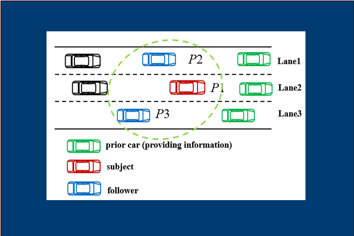
In the present study, we formulate a vehicle to execute a game that has three players as shown in Figure 1: the subject vehicle itself, serving as the leader vehicle and the two follower vehicles in the two adjacent lanes. And we also assume subject vehicle does not try to control the vehicles ahead but utilize the information from ahead.
Figure 1. Formulation of a three-person Stackelberg Game
The Stackelberg game is therefore defined as the three-person finite game with three levels of hierarchy:
Players:
P1 (1st leader), P2 (2nd leader), and P3 (follower)*
Strategies:
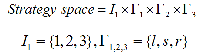
Utility design
In order to reproduce what drivers will mainly consider when they drive, we define two utility functions: basic positive utility and basic negative utility. The two utilities are related to the two factors among multiple factors that Gipps considered: speed advantage and unacceptable collision risk.
Positive utility:
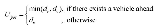
where dv denotes the visibility distance, dr the relative distance between the vehicle ahead and the subject vehicle, qa the index of the driver’s aggressiveness with a range of [0, 1].
Negative utility:
![]()
where dr denotes the relative distance between the player and the vehicle behind, vr the relative velocity, T the prediction time, and Dsuf the distance essential to change lanes.
Game Solution
The Stackelberg game solution (γ1*, γ2*, γ3*) at every instant can be obtained by solving
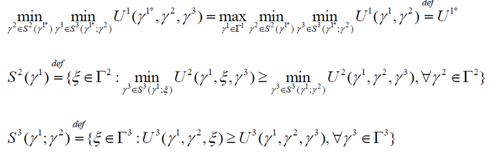
where
- U1 : the first leader’s utility, U2 : the second leader’s, and U3 : the follower’s utility
- γ1 : the possible action of the first leader, γ2 : an optimal action of the second leader forgiven γ1 , S2 : the set of γ2, γ3 : an optimal action of the follower in case that γ1 are γ2given, and S3 : the set of γ3.
- γ1*, an optimal action of the first leader. and corresponding optimal strategies of thesecond leader and the follower to γ1* are the pair (γ1*, γ2*), respectively.
Model Validation
We test a specific scenario consisting of two vehicles, in addition to the three front dummy vehicles that form a boundary of the simulation area. The purpose of the scenario is to focus on the interaction between two vehicles when they use the Stackelberg game theoretic decision model. The collision possibility Icol between vehicles is calculated by eq.1 to study the simulation
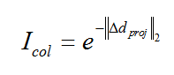
where Δdproj is the gap of the two rectangles calculated by Separating Axis Theorem as in Figure 2
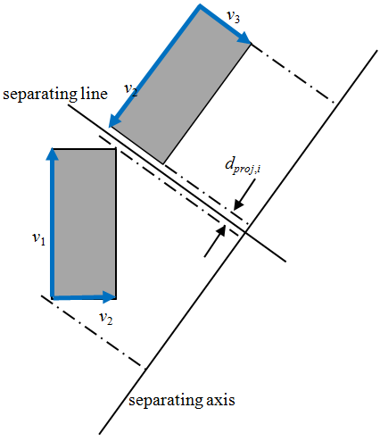
Figure 2. Separating axis theorem
Two-car unit test
Unit test scenarios:
We test a specific scenario consisting of two vehicles, in addition to the three front dummy vehicles that form a boundary of the simulation area as in Figure 4. The purpose of the scenario is to focus on the interaction between two vehicles when they use the Stackelberg game theoretic decision model. The initial condition of two vehicles is given in Table 1.
Table 1. The initial positions of the vehicles in the two vehicles test case
| Initial Condition | |||
| x0 (m) | y0 (m) | v0 (km/h) | |
| Vehicle 1 | 3.3 | 0 | 100 |
| Vehicle 2 | 6.6 | -50 | 130 |
There are four aggressiveness combinations to be tested for Vehicle 1 and 2. The test cases 1 to 4 represent the interactions of two normal drivers, an aggressive driver and a timid driver, two aggressive drivers, and two timid drivers in that order.
Unit test result:
The unit test results with a specific setting are shown in Figure 3. Panels (a), (b), (c), and (d) depict the results corresponding to the test cases mentioned before.
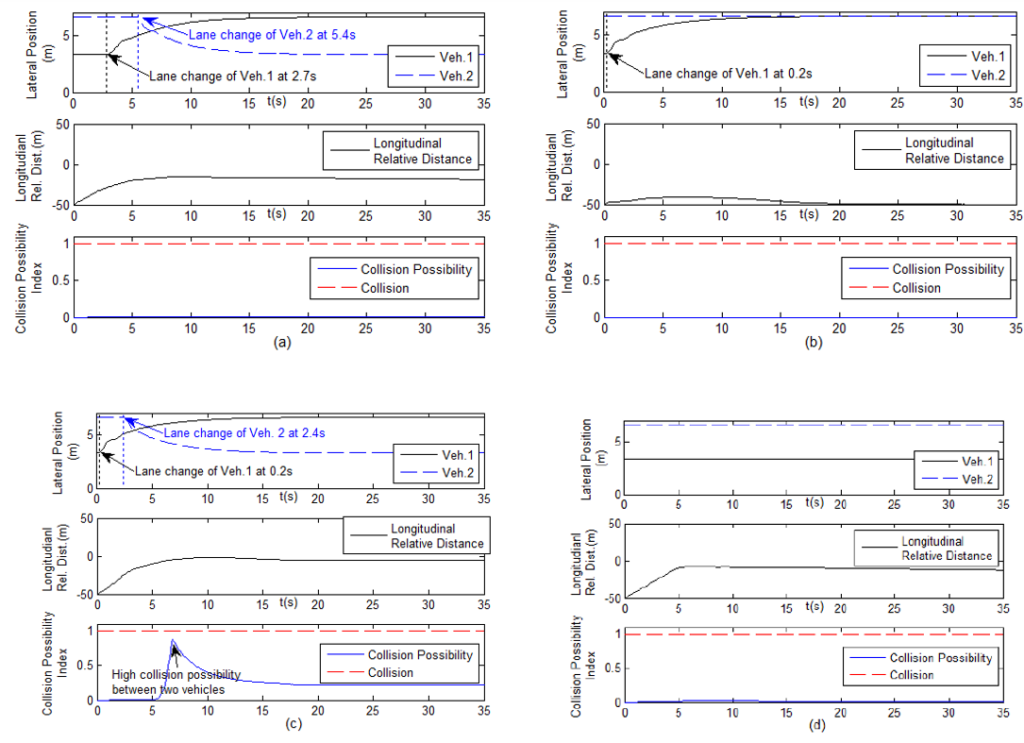
Figure 3. Unit test simulation result
The two normal driver test case (a) and the two aggressive driver test case (c) show that the driver of Vehicle 1 in the second lane changes its lane to the third lane, which initially has a larger space in front, and then Vehicle 2 changes its lane to the second lane because its free space is now restricted by Vehicle 1. Compared with Case (a), Case (c) shows that the aggressive drivers’ lane changes happens sooner than the normal drivers’. In Case (b), the timid driver of Vehicle 2 does not try to overtake the aggressive driver’s and maintains a safer relative distance. In Case (d), the combination of the two timid drivers, no drivers changes their lane. The most dangerous instant comes from Case (c). The reason for this result is that the more aggressive the drivers are, the smaller the headway they set.
Monte Carlo simulation
The above results of unit tests indicate that the interaction among the vehicles depends on the level of aggressiveness of the drivers, as well as the initial conditions of the vehicles. In order to determine the general effects of the aggressiveness of the drivers, we perform a Monte Carlo simulation involving randomized longitudinal positions and construct a model that estimates the collision possibility given the longitudinal positions and aggressiveness combinations of the drivers. We test 100 cases with random longitudinal positions of the two vehicles. The longitudinal positions of Vehicle 1 and 2 are uniformly distributed in the range of 0 to 50 m and 0 to -50 m, respectively. Three aggressive combinations (Normal/Normal, Aggressive/Timid, and Aggressive/Aggressive) are demonstrated; the case that both drivers are timid has no meaningful results. Figure 4 shows the number of potential collisions at every second.
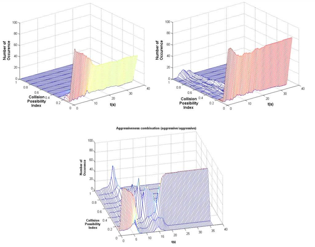
Figure 4. Monte Carlo simulation results for combined and velocity tracking controller
ANFIS modeling
ANFIS (Adaptive Neuro-Fuzzy Inference System) is a nonlinear modeling method that employs two complementary techniques: neural networks and fuzzy logic. Neural networks provide adaptive learning that fuzzy logic can use for linguistic expression via if-then rules. Using ANFIS, we build a comprehensive model to represent the vehicles‟ potential collisions according to the vehicles‟ relative position and aggressiveness combinations. We use Monte Carlo simulation results to associate collision possibilities with given relative positions and aggressive combinations.
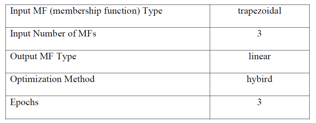
The collision possibility model is learned from two inputs and one output. Two inputs are the initial longitudinal relative positions and aggressiveness combinations. We define aggressiveness combinations (Normal/Normal, Aggressive/Timid, and Aggressive/Aggressive) as Mode 1, 2, and 3, respectively. The output used is the highest collision possibility value of every test case. The setting for the ANFIS is listed in Table 2.
Table 2. ANFIS settings in MATLAB
The ANFIS model is trained with one fourth of the data with a training error, 2%. When the model is tested with the total data, the modeling error is 6%. The error mainly occurs in Mode 2. However, the model is sufficient to show the tendency of the collision possibility as shown in Figure 5. Figure 6 shows the collision possibility model. At the combination of two normal drivers (Mode 1), the collision possibility remains low even though it increases to 0.25 when the relative distance is less than 50 m. However, if one driver becomes aggressive and another driver becomes timid, the collision possibility when the relative distance is less than 50 m increases to 0.8. Moreover, if both drivers are aggressive, the collision possibility stays at the highest level, regardless of the relative distance.
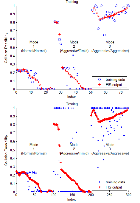
Figure 5. ANFIS training and testing results
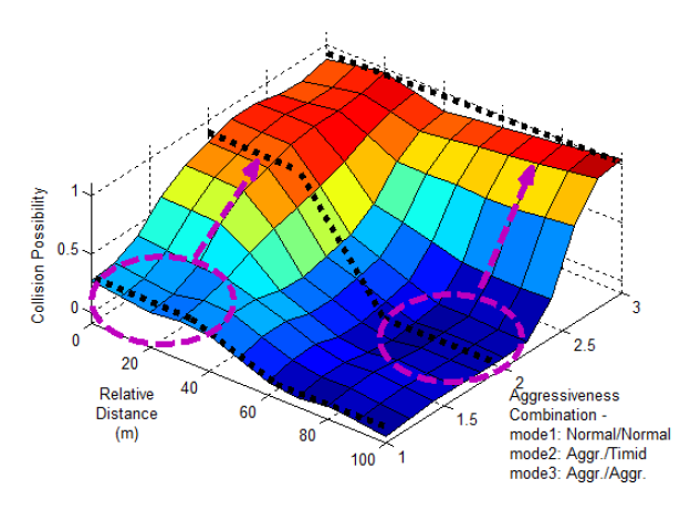
Figure 6. Rule surface of ANFIS collision possibility model
Traffic flow simulation
The Stackelberg game based highway driver decision model is used as the basis for a microscopic traffic simulation. To accomplish this, we conduct multiple vehicle simulations for the evaluation of the crash occurrence and the cumulative collision possibility according to the drivers‟ aggressiveness combinations. A 200 m section of a three-lane highway is simulated as shown in Figure 7. The density of the vehicle in the section is maintained at 10 veh/section, the flow rate 100 veh/min.
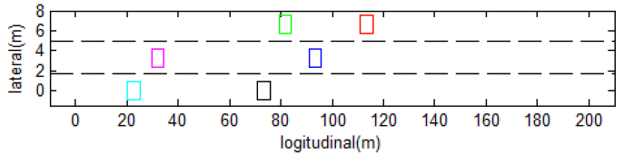
Figure 7. Configuration of the traffic flow simulation
To validate the traffic unsafety (i.e. crashes) that Stackelberg game based driver decision model leads to according to the driver’s aggressiveness, we compare the result of the traffic simulation results based on our driver decision model with the crash data from (Dingus, T et al, 2006). The occurrence of crash is counted in our result when the collision possibility index is 1. Also, when the collision possibility index exceeds 0.5, near crash is counted. The density of the traffic is 6 vehicle /section. In inattentive case, one driver is set to be aggressive (75%).
To compare the rate of crash, the occurrence of crash is converted to rate per MVMT (Million Vehicle Miles Traveled). The comparison shows a certain level of effectiveness of the model in representing the traffic unsafety, as shown in Figure 8. The results of the model have a similar level of over-approximation to the field data.
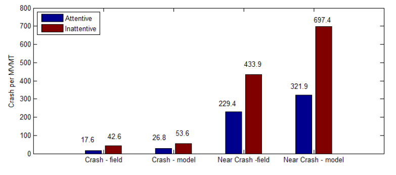
Figure 8. Comparison of crash rate
The cumulative collision possibility results are presented in Figure 9. To evaluate the effects of aggressive drivers, the ratio of aggressive drivers is set to 50% and 100% in the test cases of Aggressive/Timid and Aggressive / Aggressive in Figure 9. 5, 50, 500 runs of the simulation with the density of 6 vehicle/section yield 30,300, and 3000 vehicles simulation. 40, 400 and 4000 vehicles resulted from 8 vehicle /section. Bars in each figure show the difference caused by different drivers’ aggressiveness.
It can be seen that aggressiveness combinations influence the accumulated collision possibility regardless of the number of vehicles. Similar to the previous result, the collision possibility shows the growing tendency as the ratio of aggressive drivers increase. Also, when the density of the vehicle is higher in Figure 9 (b) compared with (a), the collision possibility increases in every aggressiveness combination, which means shorter relative distances escalate the collision possibility as described in the previous ANFIS model.
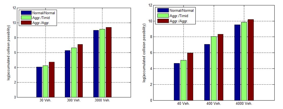
Figure 9. Distribution of cumulative collision possibilities
Finally, our ANFIS result and the application to the traffic flow simulation of the Stakelberg game based driver model imply a natural result that aggressiveness of drivers and traffic densities impact traffic safety, observed by other researchers (Whitlock, F.A. et al., 1971; Shinar, D. et al., 2004), which shows the effectiveness of our more realistic driver model. This validation step is intended to facilitate the use of this model in assessing the impact of implementation of naturalistic driving models for autonomous vehicles. Other uses of this model may include driver education campaigns and policy analysis for transportation systems.
2. Vehicle Mandatory Lane Change Model Predictive Control-a Cooperative Differential Game Approach:
Autonomous driving has become a hot research subject in nowadays. However, to achieve a human-like driving behavior, autonomous vehicle must predict accurately surrounding vehicles’ intention if no V2V exists. While many researchers relies on probabilistic methods to do so, we use game theory to study this kind of problem. Game theory has been widely used to study human interaction since it was created. We believe it would be a great tool to predict human driver’s behavior.
We now focus on a mandatory lane change scenario. Two vehicles running on a two-lane road (Fig.1). S and C mean the subject vehicle and competing vehicle respectively. We need to determine an optimal control input of both vehicle S and vehicle C to complete the cooperative mandatory lane change. For now we only control longitudinal motion and suggest a predetermined lateral motion of vehicle S. Vehicle S can choose either accelerate or decelerate to achieve a desired gap, while the vehicle C doing the opposite.
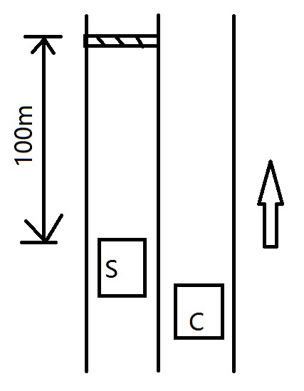
Figure 1. MLC scenario
To successfully perform an MLC, we suggest the goal of both vehicles is to achieve an acceptable gap while applying as less acceleration as possible. Since we include the cost of N steps in simulation, so the problem is a constrained model predictive optimal control problem.
QP solver is used to find the optimal control sequence and the final simulation is shown in Fig.2 and Fig.3.
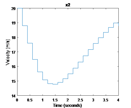
Velocity of vehicle S
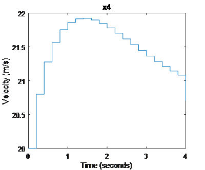
Velocity of vehicle C
Figure 2. states trajectory that vehicle S’s decelerating to achieve a gap
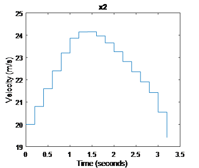
Velocity of vehicle S
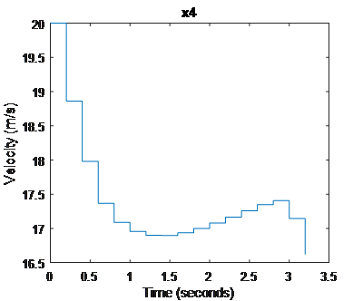
Velocity of vehicle C
Figure 3. states trajectory under scenario that vehicle S’s accelerating to achieve a gap
In Fig.2, we can tell that vehicle S decelerate to achieve a gap while vehicle C accelerate to cooperate with vehicle S, while Fig.3 indicates both vehicles are doing the opposite to achieve a gap.
We are working to add lateral motion, Connect pre-MLC and post-MLC behavior with hybrid system theory, Consider non-straight lane and Consider non-cooperative differential game.